
Orderers#
An orderer turns phase-space tracers (positions, velocities) into an
ordered result that the autoencoder consumes unchanged. All orderers share one
interface — AbstractOrderer — and return a
unified OrderingResult, so they are
interchangeable at call sites:
import phasecurvefit as pcf

orderer = pcf.orderers.MSTOrderer(k=10, jump_cap=3.0)
result = orderer.order(qs, ps)  # or: pcf.order(qs, ps, orderer)
model = pcf.nn.PathAutoencoder.make(normalizer, gamma_range=result.gamma_range, key=key)
ae, *_ = pcf.nn.train_autoencoder(model, result, config=cfg, key=key)
Choosing an orderer#
Orderer |
Best for |
Mechanism |
|---|---|---|
|
open streams; multi-petal / self-intersecting curves where a coherent velocity field can be followed |
velocity-following greedy walk from a start point |
|
near-closed loops and self-overlapping streams where the velocity field reverses and a single walk cannot traverse the arc |
kNN graph → minimum spanning tree → longest-path (diameter) backbone → arc-length ordering |
The two are complementary. The walk needs a start point and follows the flow; it covers only one arm when the velocity reverses at a progenitor. The MST needs no progenitor — the graph diameter finds the two tips itself — and orders tip-to-tip with bounded per-step jumps, which is exactly what a near-closed loop needs.
LocalFlowOrderer#
The LocalFlowOrderer is the velocity-following
greedy walk — the original phasecurvefit ordering algorithm, now behind the
orderer interface. From start_idx it repeatedly steps to the nearest unvisited tracer
under a pluggable phase-space metric, tracing the coherent flow of the
velocity field. Unlike the MST it is fully JAX-traceable (jit / vmap / grad).
import jax.numpy as jnp

import phasecurvefit as pcf

pos = {"x": jnp.linspace(0.0, 5.0, 20), "y": jnp.zeros(20)}
vel = {"x": jnp.ones(20), "y": jnp.zeros(20)}

walk = pcf.orderers.LocalFlowOrderer(metric_scale=1.0, start_idx=0)
res = walk.order(pos, vel)
assert int(res.n_visited) == 20
The hyperparameters (carried by the orderer object) are:
metric_scale— the metric’s scale parameter (e.g. the momentum weight for the defaultAlignedMomentumDistanceMetric).config— aWalkConfigcomposing the distance metric with the neighbor-query strategy (brute force, orKDTreefor large datasets). See the Metrics guide.start_idx— index of the starting tracer.direction—"forward"follows the velocity field,"backward"traces against it, and"both"walks each way fromstart_idxand stitches the two arms into one tip-to-tip ordering.max_dist— gap detection: stop when the nearest unvisited tracer is farther than this (the rest are left unvisited for the autoencoder to fill).terminate_indices,n_max— optional stopping conditions.
Because the walk follows a coherent flow, it is the right choice for open
streams and for self-intersecting curves where the velocity stays coherent
through the crossings. Its one blind spot is a near-closed loop whose velocity
reverses at a progenitor: a single walk then covers only one arm — which is
exactly where the MSTOrderer takes over. For the walk’s
mathematics, the metric internals, and the direction="both" / combine_results
machinery, see the Algorithm guide.
MSTOrderer#
The MST is host-side (NumPy/SciPy): order() is a one-shot preprocessing
step, not a jit/vmap-traceable function. Pure-spatial is the default:
import jax.numpy as jnp

import phasecurvefit as pcf

pos = {"x": jnp.linspace(0.0, 5.0, 20), "y": jnp.zeros(20)}
vel = {"x": jnp.ones(20), "y": jnp.zeros(20)}
res = pcf.orderers.MSTOrderer(k=5, jump_cap=1.0).order(pos, vel)
assert res.gamma_range == (-1.0, 1.0)
assert int(res.n_visited) == 20
jump_cap severs edges longer than its value before building the MST; it should
exceed the typical inter-tracer spacing but stay below the loop-opening /
arm-separation scale. If the kNN graph is disconnected (e.g. jump_cap too
small), on_disconnected controls the response: "raise" (default), "warn"
(order the largest component, leave the rest unvisited), or "largest" (same,
silently).
Velocity is opt-in#
Three mechanisms bring velocity into the MST (all off by default), each reusing
the phase-space notion of velocity alignment cos(v_i, v_j):
velocity_weight— edge weights become||dq|| + velocity_weight * (1 - cos(v_i, v_j)), so spatially-close arms that move oppositely are not bridged. Set it on the scale of the inter-tracer spacing.sever_cos_threshold— drop edges withcos(v_i, v_j)below the threshold, cutting the reversal seam of a near-closed loop (or cross-branch edges at a self-intersection).orient_by_velocity— flip the ordering sogammaincreases along the mean velocity, giving a deterministic, physically-meaningful direction.
For heavily self-intersecting curves (many crossings), velocity-awareness is
necessary to stop the spatial MST from short-circuiting across branches — but
such multi-petal curves are usually better served by the momentum
LocalFlowOrderer. The MST’s sweet spot is the
near-closed single loop.
Physical units (unxt)#
Orderers accept unxt.Quantity inputs and return Quantities, given a unit
system:
result = orderer.order(qs, ps, metadata=pcf.StateMetadata(usys=usys))
Because the MST is host-side, unit handling is a simple strip-in / reattach-out:
positions/velocities keep their input units and backbone is returned in the
position units. velocity_weight and jump_cap are interpreted in the usys
length units.
Result: OrderingResult#
Both orderers return one unified type. Its __call__ interpolates positions from
the ordering parameter gamma: along the backbone polyline when one is present
(MST), otherwise along the ordered visited observations (walk). The historical
WalkLocalFlowResult is a thin subclass of OrderingResult.