Ordering a Self-Intersecting Epitrochoid with the MST Backbone

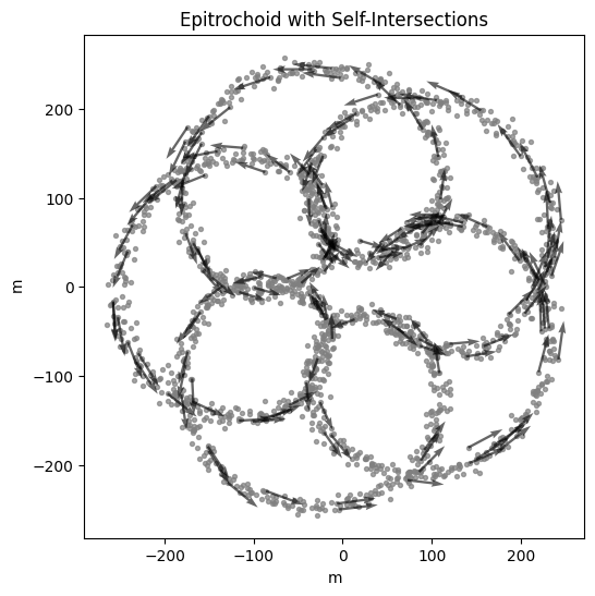
The MSTOrderer orders tracers along the longest path (graph diameter) of the minimum spanning tree of a kNN graph. It needs no start point — the diameter finds the two tips itself. This notebook uses the self-intersecting epitrochoid from the other tutorials to show a subtlety:

1. a spatial MST short-circuits across the self-intersections, and

2. a velocity-aware MST (severing anti-parallel edges) is needed to keep the ordering on a coherent branch.

The takeaway: velocity information is necessary on self-overlapping curves. (For heavily multi-petal curves the momentum LocalFlowOrderer is often the better tool; the MST’s sweet spot is the near-closed single loop.)

import jax
import jax.random as jr
import matplotlib.pyplot as plt
import numpy as np
from scipy.spatial import cKDTree

import quaxed.numpy as jnp
import unxt as u

import phasecurvefit as pcf

key = jr.key(201030)
usys = u.unitsystems.si

Data: Self-Intersecting Epitrochoid Curve

def make_self_intersecting_stream(
    key,
    *,
    n: int,
    noise_sigma=0.5,
    scale=120.0,
    R: float = 5.0,
    r: float = 1.0,
    d: float = 4.5,
):
    """Return (t, pos, vel) for an OPEN curve with self-intersections."""
    # Single outer rotation: 5° to 355° with a 10° gap
    t_start = 5.0 * jnp.pi / 180.0
    t_end = 355.0 * jnp.pi / 180.0
    t = jnp.linspace(t_start, t_end, n)

    ratio = (R + r) / r  # internal rotations per outer rotation
    x0 = scale * ((R + r) * jnp.cos(t) - d * jnp.cos(ratio * t)) / 5.0
    y0 = scale * ((R + r) * jnp.sin(t) - d * jnp.sin(ratio * t)) / 5.0

    # Derivatives for velocity
    dx0 = scale * (-(R + r) * jnp.sin(t) + d * ratio * jnp.sin(ratio * t)) / 5.0
    dy0 = scale * ((R + r) * jnp.cos(t) - d * ratio * jnp.cos(ratio * t)) / 5.0

    kx, ky = jr.split(key)
    x = x0 + noise_sigma * jr.normal(kx, (n,))
    y = y0 + noise_sigma * jr.normal(ky, (n,))

    pos = {"x": u.Q(x, usys["length"]), "y": u.Q(y, usys["length"])}
    vel = {"x": u.Q(dx0, usys["speed"]), "y": u.Q(dy0, usys["speed"])}
    return t, pos, vel

key, subkey = jr.split(key)
t, pos, vel = make_self_intersecting_stream(subkey, n=2048, noise_sigma=6)

# shuffle so the input order carries no ordering information
key, subkey = jr.split(key)
order = jr.permutation(subkey, jnp.arange(len(t)))
qs = jax.tree.map(lambda a: a[order], pos)
ps = jax.tree.map(lambda a: a[order], vel)
t_shuffled = t[order]

_fig, ax = plt.subplots(figsize=(6, 6))
ax.scatter(qs["x"], qs["y"], color="gray", alpha=0.7, s=8)
every = 12
ax.quiver(
    np.array(qs["x"][::every]),
    np.array(qs["y"][::every]),
    np.array(ps["x"][::every]),
    np.array(ps["y"][::every]),
    scale=10_000,
    width=0.005,
    alpha=0.6,
    color="black",
)
ax.set(aspect="equal", title="Epitrochoid with Self-Intersections")
plt.show()

A helper: how well is the ordering monotone in the true parameter?

We know the true curve parameter t, so we can score any ordering by the rank correlation between position-in-order and true t (|rho| ≈ 1 is perfect).

def rho(result):
    to = np.asarray(t_shuffled)[np.asarray(result.ordering)]
    r = np.corrcoef(np.arange(to.size), to)[0, 1]
    cov = int((result.indices >= 0).sum())
    return abs(r), cov


def plot_order(result, title):
    _fig, ax = plt.subplots(figsize=(7, 7))
    ax.scatter(qs["x"], qs["y"], s=3, c="lightgray")
    oq = {k: v[result.ordering] for k, v in result.positions.items()}
    timeline = np.linspace(-1, 1, len(result.ordering))
    im = ax.scatter(oq["x"], oq["y"], s=25, c=timeline, cmap="RdYlBu")
    ax.plot(oq["x"], oq["y"], c="k", lw=0.7, alpha=0.6)
    plt.colorbar(im, ax=ax, label="ordering gamma")
    r, cov = rho(result)
    ax.set(aspect="equal", title=f"{title}\n|rho|={r:.2f}, coverage={cov}/{len(t)}")
    plt.show()

1. Spatial MST — and why it short-circuits

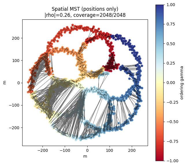
We set jump_cap from the data (a few times the median nearest-neighbour distance). With positions only, the MST happily bridges the two branches wherever they cross, so the arc-length ordering jumps between branches.

P = np.stack([np.asarray(u.ustrip(usys, qs[c])) for c in ("x", "y")], axis=1)
med = float(np.median(cKDTree(P).query(P, k=2)[0][:, 1]))

spatial = pcf.orderers.MSTOrderer(k=16, jump_cap=6.0 * med, on_disconnected="largest")
res_spatial = spatial.order(qs, ps, metadata=pcf.StateMetadata(usys=usys))
plot_order(res_spatial, "Spatial MST (positions only)")

2. Velocity-aware MST — cutting anti-parallel edges

At a crossing the two branches travel in different directions, so their velocity alignment cos(v_i, v_j) is low. sever_cos_threshold drops those edges, so the MST stays on a coherent branch. The anti-parallel edges at the crossings are exactly the ones the spatial MST used to cheat, so severing them recovers a clean ordering at essentially full coverage. (On sparser data severing can fragment the graph; on_disconnected then decides what to do — here we keep the largest component to be safe.)

velaware = pcf.orderers.MSTOrderer(
    k=16,
    jump_cap=8.0 * med,
    sever_cos_threshold=0.9,
    orient_by_velocity=True,
    on_disconnected="largest",
)
res_vel = velaware.order(qs, ps, metadata=pcf.StateMetadata(usys=usys))
plot_order(res_vel, "Velocity-aware MST (severing)")

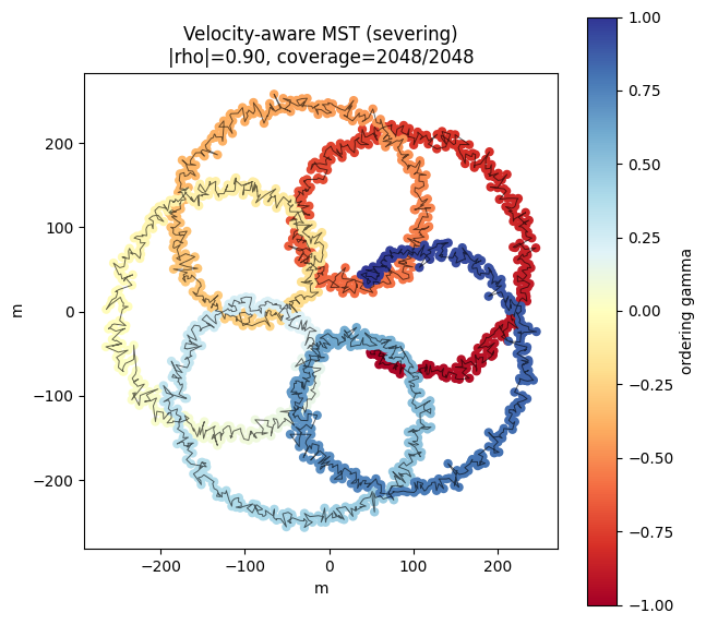
The velocity-aware ordering follows a single coherent strand cleanly (|rho| jumps from ~0.26 to ~0.9), while the spatial MST zig-zags across branches. This is the sense in which velocity is necessary for self-overlapping curves.

That said, a heavily multi-petal rose is not the MST’s natural home: the momentum LocalFlowOrderer follows such a curve directly. The MST is at its best on a near-closed single loop, where the velocity field reverses at the progenitor and a single walk cannot traverse the arc — there the MST orders tip-to-tip with no tuning at all.

3. Feeding the ordering to the autoencoder

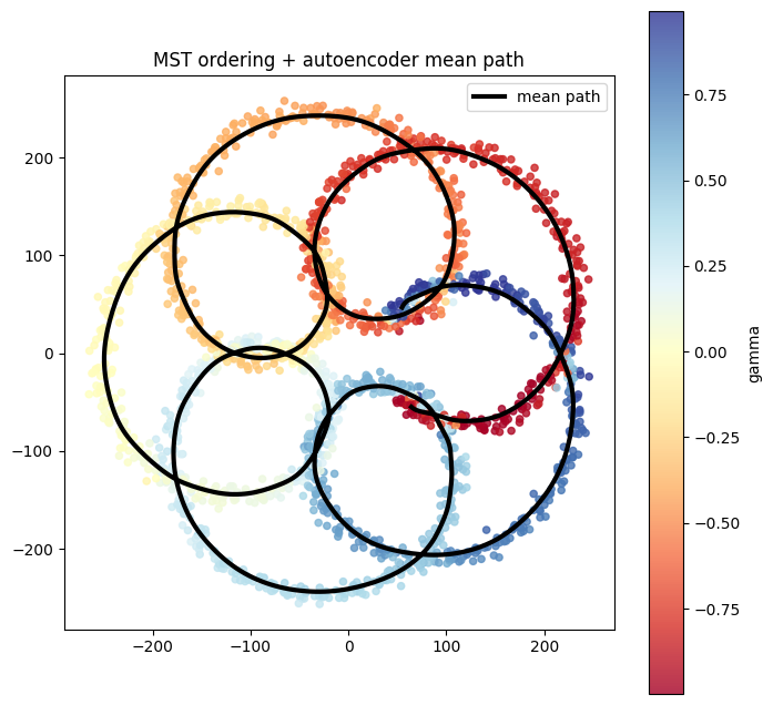
The autoencoder has two halves: an encoder mapping each tracer to its ordering parameter \(\gamma\), and a decoder mapping \(\gamma\) back to a position (the smooth “mean path”). Training runs in three phases - encoder, decoder, then a joint phase.

Two choices matter for a self-intersecting curve like this one:

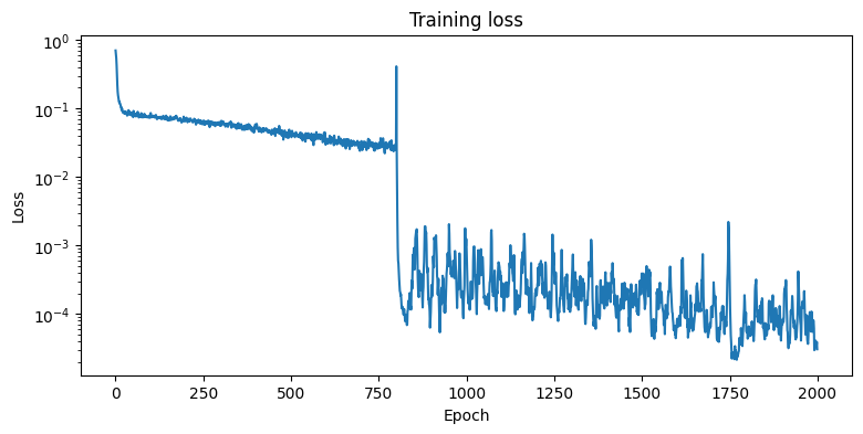
• Decoder architecture. A 5-petal rose passes through its centre five times, so the decoder \(\gamma \to (x, y)\) must make five sharp out-and-back excursions. A plain MLP (TrackNet) over-smooths these into a rounded blob. We instead use FourierTrackNet, which feeds Fourier features \([\gamma, \sin(\pi k\gamma), \cos(\pi k\gamma)]\) (\(k = 1 \dots K\)) to the MLP, giving it the high-frequency capacity to render the petals. The decoder is fully swappable via PathAutoencoder.make(decoder=...).

• The joint phase. The joint (“both”) phase optimises a different composite objective (membership + velocity alignment), which on this hard topology inflates the reported loss without improving the geometry. We set n_epochs_both=0 and stop after the decoder phase, whose spatial reconstruction is best here.

key, model_key, train_key = jr.split(key, 3)
enc_key, dec_key = jr.split(model_key)
normalizer = pcf.nn.StandardScalerNormalizer(qs, ps)

# Fourier-feature decoder: high-frequency capacity for the sharp petal excursions
# (a plain TrackNet over-smooths a 5-fold self-intersection).
decoder = pcf.nn.FourierTrackNet(
    out_size=2, n_frequencies=12, width_size=256, depth=4, key=dec_key
)
ae_model = pcf.nn.PathAutoencoder.make(
    normalizer, gamma_range=res_vel.gamma_range, decoder=decoder, key=enc_key
)

# Stop after the decoder phase (see above): no joint phase on this hard topology.
config = pcf.nn.TrainingConfig(
    n_epochs_encoder=800, n_epochs_decoder=1200, n_epochs_both=0
)
result, _, losses = pcf.nn.train_autoencoder(
    ae_model, res_vel, key=train_key, config=config
)

_fig, ax = plt.subplots(figsize=(9, 4))
ax.plot(np.asarray(losses))
ax.set(xlabel="Epoch", ylabel="Loss", yscale="log", title="Training loss")
plt.show()

_fig, ax = plt.subplots(figsize=(8, 8))
all_gamma, all_probs = result.model.encode(res_vel.positions, res_vel.velocities)
qs_pred = result(jnp.linspace(*result.gamma_range, 1_000))
im = ax.scatter(
    np.asarray(qs["x"]),
    np.asarray(qs["y"]),
    s=20,
    c=np.asarray(all_gamma),
    cmap="RdYlBu",
    alpha=0.8,
)
ax.plot(
    np.asarray(qs_pred["x"]), np.asarray(qs_pred["y"]), c="k", lw=3, label="mean path"
)
plt.colorbar(im, ax=ax, label="gamma")
ax.set(aspect="equal", title="MST ordering + autoencoder mean path")
ax.legend()
plt.show()